VisNow data model
All VisNow modules operate on data types. Modules have input ports, output ports or both. Each input port needs as an input source a data of some particular type. Similarly each output port produces data of some type.
There are few different data types in VisNow: field, geometry object and basic data types.
VisNow field
Main data type in VisNow is VisNow field (or just field).
VisNow field can represent data obtained from physical experiments, simulations and measurements, both time-dependent and static. Data may come from many different areas like fluid dynamics, medical data, weather records, engineering, etc.
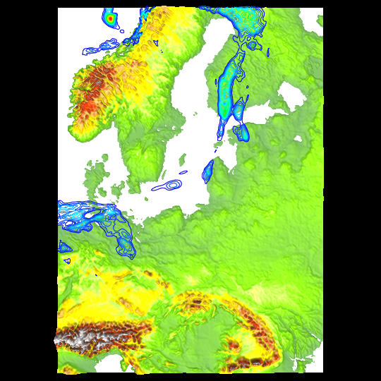
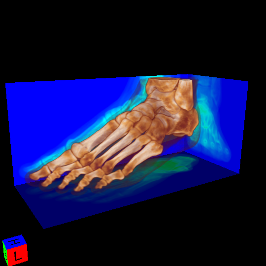
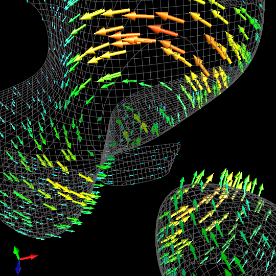
VisNow field examples
 |
 |
 |
|---|---|---|
| Meteorological | Medical (CT) | Sample vector field |
In general VisNow field is a set of atom elements (geometry) with some particular properties (components). There are two main types of field:
- regular field - where atom elements are points on the grid;
- irregular field - where atom elements are basic geometric figures and bodies called cells;
Regular fields can be loaded and stored in files with .vnf extension.
[Hint: In workspace area:
- module ports that represent field are colored in light blue, dark blue or violet;
- to see field details select: right mouse button on field port / ShowContent. This will be called “content window” later on]
Sample regular field - atom elements are points
 |
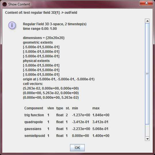 |
|---|---|
| Sample regular field | Corresponding content window |
Sample irregular field - atom elements are triangles
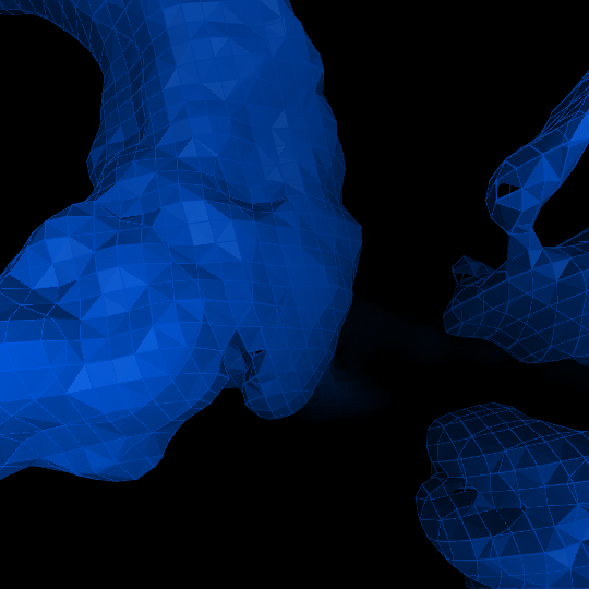 |
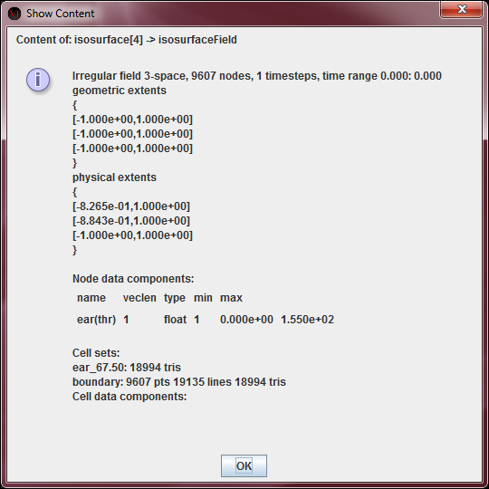 |
|---|---|
| Sample irregular field | Corresponding content window |
VisNow fields are built like on the charts above:
There are two top-level elements of field: geometry and values (otherwise called components).
I. Geometry
Geometry is representation of field in space (where space can be 2 or 3 dimensional; 2D space is less common but it still appears in some modules e.g., AVS reader, Image reader).
Field is always finite. It consists of finite number of elements and there is need to know what does every single element look like. These elements are described in structure section and their position in the space in coordinates section.
Structure
Structure describes atom elements of field. There are two different types of field: regular and irregular. And so there are two different types of structure - regular and irregular.
Case 1. Regular
Field with regular structure is composed of regular, finite lattice of points (1-, 2- or 3-dimensional). It can be square lattice generated from orthonormal basis, but it can be also generated from any other basis. Lattice can be also “bended” in a custom way (see coordinates section).
Case 2. Irregular
Field with irregular structure is composed of finite number of cells, which are geometric figures and bodies. These can be:
- 0-dimensional (points);
- 1-dimensional (segments);
- 2-dimensional (triangles, quads);
- 3-dimensional (tetrahedrons, pyramids, prisms, hexahedrons).
All these figures and bodies are built on vertices.
Each cell is a part of exactly one cell set which typically describes some particular piece of the model. For example, if one wants to simulate air flow around wing of the airplane, there will be most likely at least two cell sets: one for wing and one for air around it, which have different physical properties.
Coordinates
Coordinates describe how to arrange atom elements of the field in space.
Case 1. Regular
Regular field is in general a finite lattice of points. Coordinates of these points can be defined in two ways:
- explicitly: where every single point has it's own coordinates defined independently. This allows us to “bend” the lattice. In content window this is called “with explicit coordinates”;
- generated from basis: coordinates of every single point is calculated from basis vectors (in content window they're called “cell vectors”) and origin vector (in content window it's called “origin”). If origin vector is not defined then [0,0,0]T is taken. If basis vectors are not defined then the standard orthonormal basis is taken.
Case 2. Irregular
In this case coordinates are always defined explicitly. So every single vertex has it's own coordinates defined independently. Vertices build cells of irregular field (vertices are called “nodes” in content window).
II. Values / Components
Apart from geometry there is also data part which describes state or property of every single element of the field. This can be for example, density, energy, speed, momentum, temperature, altitude, wind, etc. So for each point or cell there is a value which describes this element. This can be scalar quantity (e.g., density, temperature) or vector quantity (e.g., momentum, speed). Additionally, property can be of different numeric type (byte, short, int, float, double, complex) logic type (true / false) or text. These properties are called otherwise components.
Case 1. Regular
Regular field case is simple. For every component there is one value for one point on the field.
Case 2. Irregular
In irregular field each component describes either vertices or cells from some particular cell set.
III. Advanced
- Each cell of irregular field (especially 2-dimensional cells) has orientation (front / back side).
- Each element of field may have optional mask (visible / invisible).
-
VisNow field can change over time. Such time-dependent field is organized in time-frames within some arbitrary time range. Frames don't need to be uniformly distributed over time, instead, each frame is described by a single real number which denotes its position on time axis. Only some parts of field can change over time, that is:
- coordinates of points / vertices (but only in case if they are defined explicitly);
- mask (so one can show / hide elements over time);
- values / components (change of state / property of the element over time – typical in all time-based simulations).
Data between frames is linearly interpolated. Data outside given time range is taken from the boundary. In content window, time data occurrence is denoted by “time range” and “st.” (abbreviation for “number of steps”).
-
Regular fields support tiles. Tiles are typically used when some large data set is split into smaller, separated parts (which usually goes together with separated input files). These parts (tiles) are 1-, 2- or 3-dimensional boxes (depends on dimension of the field). Field covers one or more tiles (fully or partially).
IV. Miscellaneous
- VisNow calculates automatically basic statistics of components and boundary of irregular field (in content window as “min/max” and “boundary” respectively).
- Fields, cell sets, components may have names.
- “Geometric” and “physical extents” in content window sometimes differs which happens mostly in case of geometrical rescaling of 2D field in 3D space (used mainly in Axes3D module).
- Coordinates of points / vertices are always real numbers (32 bit float).
Geometry object
Geometry object is object passed from any module able to output some graphical content into some viewer module. There are two types of geometry objects 2D and 3D.
[Hint: In workspace area, module ports that represent geometry object are colored in red for 3D objects and in orange for 2D objects]
Basic data types
Basic data types like integer or real number are present in some modules.
[Hint: In workspace area, module ports that represent basic data types are colored in light or dark grey]